One dimensional sieve introduction

Return to MSERs and extrema

1D Signals to MSERs and granules

Matlab function IllustrateSIV_1 illustrates how MSERs (maximally stable extremal regions) and sieves are related. We start with one dimensional signals before moving to two dimensional images and three dimensional volumes.

Consider a signal, <math>X</math> X=getData('PULSES3WIDE') >blue X=0 5 5 0 0 1 1 4 3 3 2 2 1 2 2 2 1 0 0 0 1 1 0 3 2 0 0 0 6 0 0

<math>X</math> has three one-sample-wide maxima (<math>M^1_8</math> , <math>M^1_{24}</math> , <math>M^1_{29}</math> ), two two-sample-wide maxima (<math>M^2_{14}</math> , <math>M^2_{21}</math>) some of which, when removed, will persist as larger scale maxima, e.g. <math>M^1_{24}</math> will become two samples wide as the peak is clipped off.

Filter

Linear

A linear Gaussian filter with <math>\sigma=2</math> attenuates extrema without introducing new ones. But blurring may be a problem.

h=fspecial('Gaussian',9,2);
Y=conv(X,(h(5,:)/sum(h(5,:))),'same');

Non-linear: the starting point for MSER's

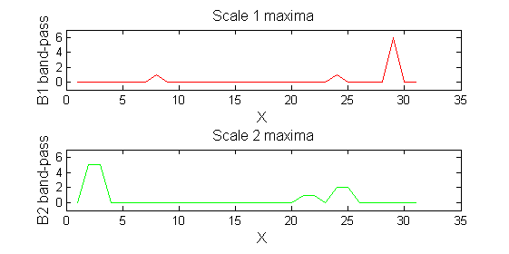
A low-pass 'o' sieve scale 1 (non-linear filter underpinning the MSER algorithm) can remove scale 1 maxima. The result is shown in red, extrema at <math>M^1_8</math> , <math>M^1_{24}</math> , <math>M^1_{29}</math> have been removed. There is no blur. The remaining signal is unchanged.

scaleA=1;
Y1=SIVND_m(X,scaleA,'o');

Scale 2 maxima are removed next using the 'o' sieve scale 2. The result is shown in green. Extrema at <math>M^2_{14}</math> , <math>M^2_{21}</math> have been removed. Still no blur and what remains is unchanged.

scaleB=2;
Y2=SIVND_m(X,scaleB,'o');

A high-pass 'o' sieve scale 1 shows the extrema that have been removed. In red the scale 1 extrema at <math>M^1_8</math> , <math>M^1_{24}</math> , <math>M^1_{29}</math> have been removed. In green extrema of scale 2 are shown. In the sieve terminology these are granules. Think of grading gravel using sieves, large holes let through large grains and small holes let through small grains. Here scale is measured as length. If granules don't fit they don't get through - unlike linear filters which leak.

red=double(X)-double(Y1); 
green=double(Y1)-double(Y2);

Repeat over scales 0 to 15

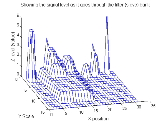
Increasing the scale (towards the front) removes extrema of increasing length. The algorithm cannot create new maxima (it is an 'o' sieve) it is, therefore, scale-space preserving.

YY=ones([length(X),1+maxscale]);
for scale=0:maxscale
    Y2=SIVND_m(Y1,scale,'o',1,'l',4);
    YY(:,scale+1)=Y2';
    Y1=Y2; % each stage of the filter (sieve) is idempotent
end

Label the granules

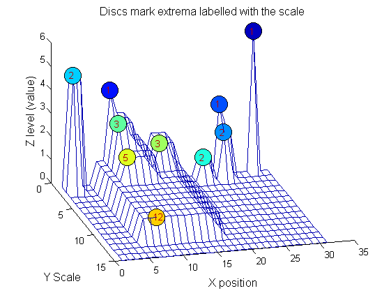
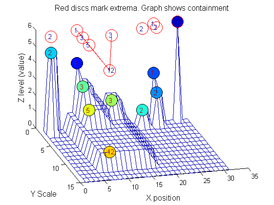
We can create a data structure that captures the properties of each granule. The number in each disc indicates the granule scale. Each cell in the PictureElement field has a list of indexes recording the granule position (<math>X</math>). (In 1D this is best done run-length coded but this code is designed to also work in 2D.)

g=SIVND_m(X,maxscale,'o',1,'g',4);
g =   Number: 10
             area: [1 1 1 2 2 2 3 3 5 12]
            value: [6 1 1 2 5 1 1 1 1 1]
            level: [6 4 3 2 5 1 3 2 2 1]
        deltaArea: [5 2 1 7 3 12 2 2 7 19]
        last_area: [6 3 2 9 5 14 5 5 12 31]
             root: [29 8 24 24 2 21 8 14 8 8]
   PictureElement: {1x10 cell}

g.PictureElement

 Columns 1 through 9

   [29]    [8]    [24]    [2x1 double]    [2x1 double]    [2x1 double]    [3x1 double]    [3x1 double]    [5x1 double]  [12x1 double]

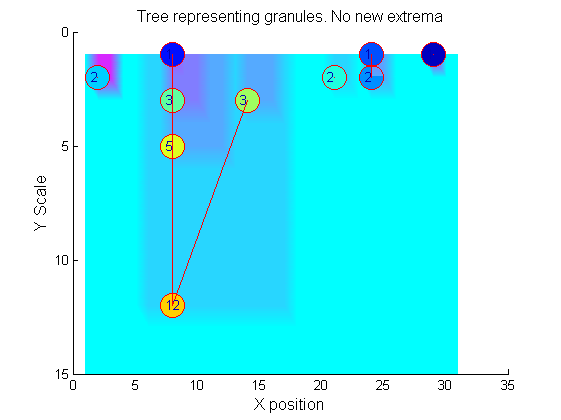
Tracing the granules through scale-space identifies candidate MSER's

The granules contain all the information in the signal. The tree illustrates the relationship between granules. The granules at <math>X=8</math> (scales 1, 3, 5, 12) indicates a region that is stable over scale. Likewise at <math>X=24</math> (scales 1, 2). One might argue that the latter is the less stable.

We have candidate 1D MSER's

Which is the most stable?

This is a pragmatic judgement. Parameters might include

1. how stable over scale (length)
2. amplitude (value or level)
3. a vector of amplitude over scale
4. proximity to others

So far maxima. What about minima and more?

The filter (sieve) that finds maxima is a connect-set opening ('o' sieve). A 'c' sieve finds the connected-set closing, or minima. To work with minima we could:

• invert the signal, process it, and invert it back.
• OR we could substitute a mini for a max:

    if type=='o'
       v=min(deltas);
   elseif type=='c'
       v=max(deltas);
   end

Actually, the SIVND_m.m implementation uses the latter. It also maintains lists of both maxima and minima throughout.