GFtbox
What is GFtbox?

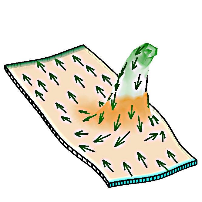
We wish to understand how patterns of gene activity in biological organs influence the developing shape. Our suggestion is that genes may regulate growth direction independently of growth rate. We formalised our ideas in the Growing Polarised Tissue Framework (Kennaway et. al. PLoS Computational Biology, in press). The icon is based on Kennaway et. al. Fig. 4 and shows an asymmetrical spur that has grown under the influence of a polariser, arrows.
Intuition is not, however, a good guide to the consequences: how patterns of growth interact with each other and a continuous sheet of material to produce complex shapes. It is therefore necessary to translate intuition into a mathematical form (as a computable model) and compute the results. Rather than writing full blown specific, custom software for each model we chose to produce a general purpose package: GFtbox within which individual computable models can be created.
GFtbox projects comprise two parts, the Mesh and the Interaction function. A loose analogy is to say that the Mesh corresponds to the cell membranes and cytoplasm (the structure) and the Interaction function corresponds to the nucleus and DNA (the regulatory system). You need both to grow - and they interact and so must be compatible with each other.
The GFtbox allowed us to test the veracity of the computational kernel using simple examples (Supplemental Text 1 in Kennaway et. al.) before building a library of examples illustrating the properties of the GPT-framework (Results in Kennaway et. al.) and embarking on modelling growing biological tissues (Green et. al.). Using GFtbox one can start with a simple sheet of tissue (the canvas), lay out experimentally observed, or hypothesised, patterns of regulator activity and then grow the canvas in 3D. Patterning can continue during growth and the final shape can be compared quantitatively with it's biological counterpart - so testing the hypotheses ( Cui et. al. ).
To work with GFtbox is to practice thinking quantitatively about the relationship between genes, growth and form.
What does GFtbox require?
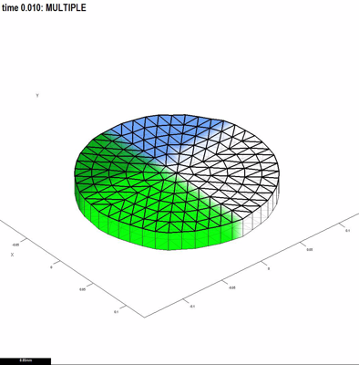
GFtbox is written in Matlab. GFtbox does not require any extra Mathworks toolboxes. Matlab is available as a 30 day free trial and there is a student edition. GFtbox comprises about 1000 subroutines and 50,000 lines of code. It has a computational kernel and lots of supporting routines that allow individual models, the part that a user sees, to be very compact - 10 to 100 lines. For example, the model shown in Fig. 1 has a mesh that was setup using the graphical user interface and interaction function code that articulates (describes) the model as follows:
   if (Steps(m)==0) && m.globalDynamicProps.doinit  % Initialisation code.
       id_a_p(m.nodes(:,1)<-0.03)=1; % setup region for A where identity factor A is represented by id_a_p
       id_b_p(m.nodes(:,2)<-0.01)=1; % setup region for B
   else
       % @@KRN Growth Regulatory Network
       kapar_p(:) = id_a_l .* inh(1,id_b_l); % growth rate
       kaper_p(:) = kapar_p; % isotropic growth
       kbpar_p(:) = kapar_p; % same on both sides of the sheet
       kbper_p(:) = kapar_p; % same
       knor_p(:)  = 0;       % thickness not growing
   end
Why Matlab? The language suits our problem - the reasoning goes like this. Tissue is represented by a thin 3D mesh. Growth factors levels vary spatially forming patterns, e.g. Fig. 1. Here there are two, A and B. We might make the hypothesis that the growth rate is specified by A but partially inhibited by B (inhibited by an amount K). This is a simple idea that can be expressed in Matlab equally simply by writing Growth=A .* inh(K, B). This is because variables A and B can represent vectors - in this case a level for each node in the mesh. We also define a general inhibition function (inh). It means that it is straightforward to convert our thoughts on the biology into a programmatic description of a computational model. Moreover, the language is well documented with lots of convenient tools. In particular, Matlab has an extensive library of portable graphical user interface (GUI) functions - and this is convenient for producing tools to visualise the mesh and patterns of growth factors.
The computational bottleneck in GFtbox is solving the finite elements equation: we find that the Matlab cgs function is quicker and more accurate than alternatives from other sources (lsqr, culaSgesvd, there are options to choose these solvers and the speed of computation is displayed constantly at the bottom of the GUI). The speed of GFtbox appears to be limited by memory-cpu bandwidth rather than cpu speed. It runs best interactively on a 64 bit machine, lots of memory and a silicon hard-drive. Growing GFtbox models does not require the GUI - we can run multiple models on a computing cluster and then visualise the results on the GUI.
Matlab is a weakly typed language and that too is an advantage whilst we develop the necessary concepts for GFtbox. (Whilst it is possible to create a dedicated class library, we defer that until we are clearer about what functionality will be needed to model most biology.) In addition, Matlab is sufficiently flexible that inexperienced programmers, half our team are biologists, can pick it up on-the-fly. It behaves as an interpreted language, which makes it easy to break and step through code to follow what is happening.
Matlab runs on Windows, Mac and Linux. It is freely available and well supported - but not free of cost. Programmers need to earn a living. We prefer our paid experts to focus on our speciality and let Mathworks maintain compatibility with new processors, OpenGL, multi-threading, algebraic algorithms (appropriate LAPACK and machine-specific BLAS libraries), user interfaces and handle multi-platform problems. The key Matlab numerical algorithms are documented and generally visible and there is a large user-base providing lots of web based help.
How to start using GFtbox
GFtbox can be freely downloaded from sourceforge. After downloading, start Matlab, cd to the GFtbox directory, and give the command GFtbox. GFtbox will start and present you with its graphic interface.
GFtbox automatically adds all of its subdirectories to the Matlab command path. If you give a savepath command at the Matlab console, then Matlab will remember where GFtbox is, and on subsequent runs of Matlab you will not have to cd to the GFtbox directory before running it.
In addition to the tutorials given here, GFtbox comes with several tutorial projects and the projects behind our published Figures. These projects appear on the Projects menu of the GFtbox window, in the Models submenu. There is a Help menu and when a new project is formed - the new associated interaction function is filled with comments that illustrate how the model can be written. In the GUI, mouseover text is provided for each of the GUI functions and the last item in every menu is a local help submenu. Documentation files can be found in the doc subdirectory of GFtbox.
Limitations of GFtbox
GFtbox is primarily for modelling curved finitely thick surfaces and does not handle bulk three-dimensional solids.
(More stuff to appear...)
