Return to MSERs and extrema
1D Signals to MSERs and granules
Matlab function IllustrateSIV_1 illustrates how MSERs (maximally stable extremal regions) and sieves are related. We start with one dimensional signals before moving to two dimensional images and three dimensional volumes.

|
Consider a signal, <math>X</math>
X=getData('PULSES3WIDE')
>blue  X=0 5 5 0 0 1 1 4 3 3 2 2 1 2 2 2 1 0 0 0 1 1 0 3 2 0 0 0 6 0 0
|
| <math>X</math> has three one-sample-wide maxima (<math>M^1_8</math> , <math>M^1_{24}</math> , <math>M^1_{29}</math> ), two two-sample-wide maxima (<math>M^2_{14}</math> , <math>M^2_{21}</math>) some of which, when removed, will persist as larger scale maxima, e.g. <math>M^1_{24}</math> will become two samples wide as the peak is clipped off.
|

|
Filter
Linear
| A linear Gaussian filter with <math>\sigma=2</math> attenuates extrema without introducing new ones. But blurring may be a problem.
|

|
h=fspecial('Gaussian',9,2);
Y=conv(X,(h(5,:)/sum(h(5,:))),'same');
Non-linear
| A low-pass 'o' sieve scale 1 (non-linear filter underpinning the MSER algorithm) can remove scale 1 maxima. The result is shown in red, extrema at <math>M^1_8</math> , <math>M^1_{24}</math> , <math>M^1_{29}</math> have been removed. There is no blur. The remaining signal is unchanged.
|

|
scaleA=1;
Y1=SIVND_m(X,scaleA,'o');
| Scale 2 maxima are removed next using the 'o' sieve scale 2. The result is shown in green. Extrema at <math>M^2_{14}</math> , <math>M^2_{21}</math> have been removed. Still no blur and what remains is unchanged.
|

|
scaleB=2;
Y2=SIVND_m(X,scaleB,'o');
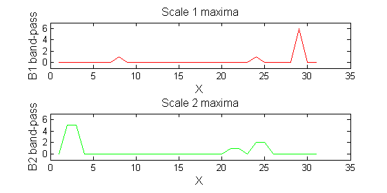
| A high-pass 'o' sieve scale 1 shows the extrema that have been removed. In red the scale 1 extrema at <math>M^1_8</math> , <math>M^1_{24}</math> , <math>M^1_{29}</math> have been removed. In blue extrema of scale 2 are shown. In the sieve terminology these are granules. Think of grading gravel using sieves, large holes let through large grains and small holes let through small grains. Here scale is measured as length.
|

|


