One dimensional sieve applied to images: Difference between revisions
Created page with "[http://cmpdartsvr3.cmp.uea.ac.uk/wiki/BanghamLab/index.php/MSER%27s_and_Connected_sets#One_dimensional_signals Return to MSERs and extrema]<br><br> =<span style="color:Chocol..." |
|||
| (27 intermediate revisions by the same user not shown) | |||
| Line 1: | Line 1: | ||
[http://cmpdartsvr3.cmp.uea.ac.uk/wiki/BanghamLab/index.php/MSER%27s_and_Connected_sets#One_dimensional_signals Return to MSERs and extrema]<br><br> | [http://cmpdartsvr3.cmp.uea.ac.uk/wiki/BanghamLab/index.php/MSER%27s_and_Connected_sets#One_dimensional_signals Return to MSERs and extrema]<br><br> | ||
=<span style="color: | ====<span style="color:Navy">'siv4.mex' implemenation applies the ''m''-sieve to a vector or column wise to a matrix</span>==== | ||
A Matlab function | A Matlab function siv4_test.m illustrates how siv4.mex can be used to analyse columns of 1D data.<br><br> | ||
{| border="0" cellpadding="5" cellspacing="5" 3D extrema thumb.gif | {| border="0" cellpadding="5" cellspacing="5" 3D extrema thumb.gif | ||
|- valign="top" | |- valign="top" | ||
| Line 12: | Line 11: | ||
{| border="0" cellpadding="5" cellspacing="5" | {| border="0" cellpadding="5" cellspacing="5" | ||
|- valign="top" | |- valign="top" | ||
|width=" | |width="30%"| The data has minima and maxima of different scales (lengths). In one dimension we measure pulse length using a ruler, measuring tape or whatever - but not frequency or Gaussian scale. | ||
|[[Image:IllustrateSIV_1_02.png|400px]] | |width="50%"| [[Image:IllustrateSIV_1_02.png|400px]] | ||
|} | |} | ||
=<span style="color:Chocolate">Filter</span>= | =<span style="color:Chocolate">Filter</span>= | ||
====<span style="color:SaddleBrown"> | ====<span style="color:SaddleBrown">Lowpass siv4.mex</span>==== | ||
{| border="0" cellpadding="5" cellspacing="5" | {| border="0" cellpadding="5" cellspacing="5" | ||
|- valign="top" | |- valign="top" | ||
|width=" | |width="30%"| Imagine that within the data above there is a signal, which may comprise positive or negative pulses, that is contaminated by smaller scale noise (leftmost panel). <br><br> | ||
|[[Image: | Then 'siv4.mex' (i.e. compiled from the 'C' to suite your operating system) can filter out the smaller scale noise - irrespective of amplitude, i.e. it removes smaller scale (length) extrema.<br><br>The rightmost panels show the results of removing all 'noise' less than scales 1, 5 and 10. Unlike linear filters edges remain well defined and 'noise' is completely removed. | ||
|width="50%"| [[Image:siv4_test_2.png|550px|Sieved]] | |||
|} | |} | ||
data{1}=siv4_alt('PULSES3WIDE',[2;5;10]); | |||
data{1} | |||
ans = | |||
y: {[34x1 double] [34x1 double] [34x1 double]} % outputs for the 3 specified scales | |||
scan: [34 34] % instructing single column processing | |||
X: [34x1 double] % input data | |||
options: [3x4 double] % options (see elsewhere) | |||
outputs: 'lll' % outputs all lowpass | |||
type: 'int' % input data may be double but only contains integers | |||
name: 'PULSES3WIDE' | |||
====<span style="color: | ====<span style="color:navy">Now what about '''scale-space'''?. </span>==== | ||
[[Image:Siv4 test 5.png|400px|center|'m' non-linear filter (sieve) compared to Gaussian filter]] | |||
{| border="0" cellpadding="5" cellspacing="5" | {| border="0" cellpadding="5" cellspacing="5" | ||
|- valign="top" | |- valign="top" | ||
|width="50%"| '''A low-pass''' ' | |width="50%"| Left Panel. '''A low-pass''' 'm' sieve can remove extrema at multiple scales. Here, siv4.m gradually removes extrema as scale increases from scale 1 to scale 64. The resulting traces are shown as a 'heat map' where the signal goes from left to right, bright colours like red are large amplitude, small scale extrema. At each increasing scale (down the map) extrema have been removed. As result, we can for example see the buried large scale, low amplitude pulse revealed in panel 4 of the previous Figure, as a light green rectangle that starts at ''n=6'' and persists to ''n=26'', i.e. ''scale=20''. <br><br> | ||
The 'm'-sieve preserves scale-space so no new extrema (light regions) are formed as we move to increasing scales.<br> | |||
|width="50%"| Right Panel. A ''Gaussian'' filter bank also preserves scale-space as shown by Witkin 1986.<br> | |||
(Babaud et. al. 1986 "The uniqueness of the Gaussian kernel ...")<ref>Babaud, Jean; Witkin, Andrew P.; Baudin, Michel; Duda, Richard O., "Uniqueness of the Gaussian Kernel for Scale-Space Filtering," Pattern Analysis and Machine Intelligence, IEEE Transactions on , vol.PAMI-8, no.1, pp.26,33, Jan. 1986 doi: 10.1109/TPAMI.1986.4767749</ref>==References== | |||
<references /> | |||
|width="50%"| | |||
|} | |} | ||
= | ====<span style="color:navy">Using ''granules'' to represent the data segment. </span>==== | ||
<span style="color: | |||
{| border="0" cellpadding="5" cellspacing="5" | {| border="0" cellpadding="5" cellspacing="5" | ||
|- valign="top" | |- valign="top" | ||
|width="50%"| | |width="50%"| Another heat-map. The plot is an alternative view of the left Panel above. This time showing the features (at each scale) that are peeled off (removed) by increasing scale sieve filters. The color map is 'jet' to make the features more visible. We call these features granules. Granules are a mapping of the original signal. Thus, the granularity domain contains all the information in the original signal. It is possible to imagine a 'tree' representation of these granules and then use some mechanism to select 'salient' granules (features). ([[One_dimensional_sieve_introduction#Tracing_the_granules_through_scale-space_identifies_candidate_MSER.27s | see here for the connection with MSER's.]]) The idea is to 'concentrate' the useful information. | ||
|width="50%"| [[Image:Siv4 test granules.png|400px|'o' non-linear filter (sieve)]] | |||
|[[Image: | |||
|} | |} | ||
An alternative is to treat the granularity domain in the manner of wavelets and concentrate the useful information by summing the 'energy' within the granules (in the signal fragment) along each scale to produce a histogram the equivalent of a local power spectrum. This can be further simplified into, say, twenty logarithmically spaced scale-bands. These two steps lose information (but hopefully concentrate useful components). To be useful, granularity spectrum should be normalised. One way is to compute the equivalent of the cepstrum. Similarly, the phase. | |||
Latest revision as of 22:55, 22 June 2014
'siv4.mex' implemenation applies the m-sieve to a vector or column wise to a matrix
A Matlab function siv4_test.m illustrates how siv4.mex can be used to analyse columns of 1D data.
Consider a signal, <math>X</math>X=getData('PULSES3WIDE')
>blue X=0 5 5 0 0 1 1 4 3 3 2 2 1 2 2 2 1 0 0 0 1 1 0 3 2 0 0 0 6 0 0
|
| The data has minima and maxima of different scales (lengths). In one dimension we measure pulse length using a ruler, measuring tape or whatever - but not frequency or Gaussian scale. | 
|
Filter
Lowpass siv4.mex
data{1}=siv4_alt('PULSES3WIDE',[2;5;10]);
data{1}
       ans =
         y: {[34x1 double]  [34x1 double]  [34x1 double]} % outputs for the 3 specified scales
      scan: [34 34]            % instructing single column processing
         X: [34x1 double]    % input data
   options: [3x4 double]   % options (see elsewhere)
   outputs: 'lll'                 % outputs all lowpass
      type: 'int'                 % input data may be double but only contains integers
      name: 'PULSES3WIDE'
Now what about scale-space?.

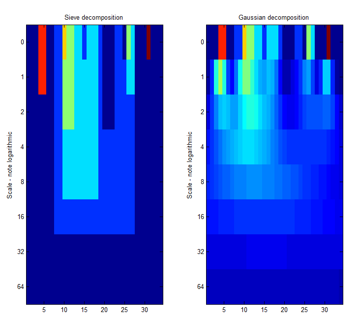
| Left Panel. A low-pass 'm' sieve can remove extrema at multiple scales. Here, siv4.m gradually removes extrema as scale increases from scale 1 to scale 64. The resulting traces are shown as a 'heat map' where the signal goes from left to right, bright colours like red are large amplitude, small scale extrema. At each increasing scale (down the map) extrema have been removed. As result, we can for example see the buried large scale, low amplitude pulse revealed in panel 4 of the previous Figure, as a light green rectangle that starts at n=6 and persists to n=26, i.e. scale=20. The 'm'-sieve preserves scale-space so no new extrema (light regions) are formed as we move to increasing scales. |
Right Panel. A Gaussian filter bank also preserves scale-space as shown by Witkin 1986. (Babaud et. al. 1986 "The uniqueness of the Gaussian kernel ...")<ref>Babaud, Jean; Witkin, Andrew P.; Baudin, Michel; Duda, Richard O., "Uniqueness of the Gaussian Kernel for Scale-Space Filtering," Pattern Analysis and Machine Intelligence, IEEE Transactions on , vol.PAMI-8, no.1, pp.26,33, Jan. 1986 doi: 10.1109/TPAMI.1986.4767749</ref>==References== <references /> |
Using granules to represent the data segment.
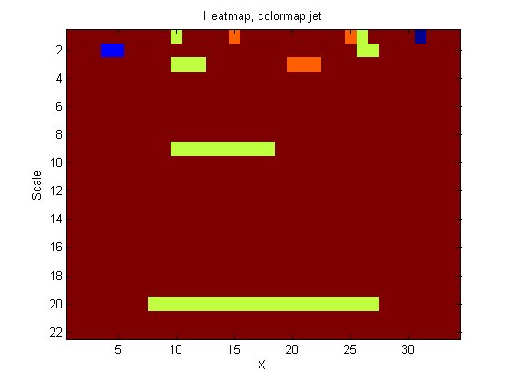
| Another heat-map. The plot is an alternative view of the left Panel above. This time showing the features (at each scale) that are peeled off (removed) by increasing scale sieve filters. The color map is 'jet' to make the features more visible. We call these features granules. Granules are a mapping of the original signal. Thus, the granularity domain contains all the information in the original signal. It is possible to imagine a 'tree' representation of these granules and then use some mechanism to select 'salient' granules (features). ( see here for the connection with MSER's.) The idea is to 'concentrate' the useful information. | 
|
An alternative is to treat the granularity domain in the manner of wavelets and concentrate the useful information by summing the 'energy' within the granules (in the signal fragment) along each scale to produce a histogram the equivalent of a local power spectrum. This can be further simplified into, say, twenty logarithmically spaced scale-bands. These two steps lose information (but hopefully concentrate useful components). To be useful, granularity spectrum should be normalised. One way is to compute the equivalent of the cepstrum. Similarly, the phase.
