One dimensional sieve introduction: Difference between revisions
No edit summary |
|||
| (2 intermediate revisions by the same user not shown) | |||
| Line 1: | Line 1: | ||
[http://cmpdartsvr3.cmp.uea.ac.uk/wiki/BanghamLab/index.php/MSER%27s_and_Connected_sets#One_dimensional_signals Return to MSERs and extrema]<br><br> | [http://cmpdartsvr3.cmp.uea.ac.uk/wiki/BanghamLab/index.php/MSER%27s_and_Connected_sets#One_dimensional_signals Return to MSERs and extrema]<br><br> | ||
=<span style="color:Chocolate">1D Signals to MSERs and granules</span>= | =<span style="color:Chocolate">1D Signals to MSERs and granules</span>= | ||
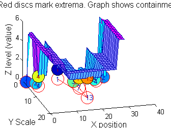
Matlab function IllustrateSIV_1 illustrates how MSERs (maximally stable extremal regions) and sieves are related. We start with one dimensional signals before moving to two dimensional images and three dimensional volumes. | A Matlab function IllustrateSIV_1.m illustrates how MSERs (maximally stable extremal regions) and sieves are related. We start with one dimensional signals before moving to two dimensional images and three dimensional volumes.<br><br> | ||
The information lies in the pattern of pulses. Each pulse is characterised by a position, length (scale) and amplitude. The goal is to find maxima that persist over a number of scales - i.e. they are stable.<br><br> | |||
{| border="0" cellpadding="5" cellspacing="5" 3D extrema thumb.gif | {| border="0" cellpadding="5" cellspacing="5" 3D extrema thumb.gif | ||
|- valign="top" | |- valign="top" | ||
| Line 20: | Line 21: | ||
{| border="0" cellpadding="5" cellspacing="5" | {| border="0" cellpadding="5" cellspacing="5" | ||
|- valign="top" | |- valign="top" | ||
|width="50%"| A linear Gaussian filter with <math>\sigma=2</math> attenuates extrema without introducing new ones. | |width="50%"| A linear Gaussian filter with <math>\sigma=2</math> attenuates extrema without introducing new ones. The signal is simpler but has blurring made large scale information more difficult to read? | ||
|[[Image:GaussianSmoothedSigma2.png|350px|Gaussian filtered]] | |[[Image:GaussianSmoothedSigma2.png|350px|Gaussian filtered]] | ||
|} | |} | ||
Latest revision as of 16:55, 3 January 2014
1D Signals to MSERs and granules
A Matlab function IllustrateSIV_1.m illustrates how MSERs (maximally stable extremal regions) and sieves are related. We start with one dimensional signals before moving to two dimensional images and three dimensional volumes.
The information lies in the pattern of pulses. Each pulse is characterised by a position, length (scale) and amplitude. The goal is to find maxima that persist over a number of scales - i.e. they are stable.
Consider a signal, <math>X</math>X=getData('PULSES3WIDE')
>blue X=0 5 5 0 0 1 1 4 3 3 2 2 1 2 2 2 1 0 0 0 1 1 0 3 2 0 0 0 6 0 0
|
Filter
Linear
| A linear Gaussian filter with <math>\sigma=2</math> attenuates extrema without introducing new ones. The signal is simpler but has blurring made large scale information more difficult to read? | 
|
h=fspecial('Gaussian',9,2);
Y=conv(X,(h(5,:)/sum(h(5,:))),'same');
Non-linear: the starting point for MSER's
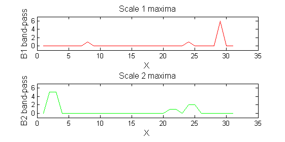
scaleA=1;
Y1=SIVND_m(X,scaleA,'o');
scaleB=2;
Y2=SIVND_m(X,scaleB,'o');
red=double(X)-double(Y1);
green=double(Y1)-double(Y2);
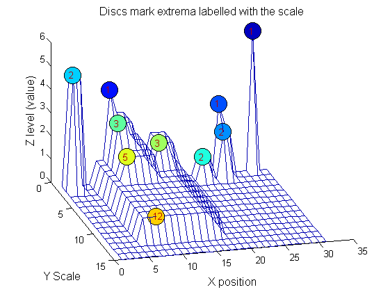
Repeat over scales 0 to 15
| Increasing the scale (towards the front) removes extrema of increasing length. The algorithm cannot create new maxima (it is an 'o' sieve) it is, therefore, scale-space preserving. | 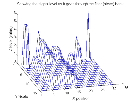
|
YY=ones([length(X),1+maxscale]);
for scale=0:maxscale
    Y2=SIVND_m(Y1,scale,'o',1,'l',4);
    YY(:,scale+1)=Y2';
    Y1=Y2; % each stage of the filter (sieve) is idempotent
end
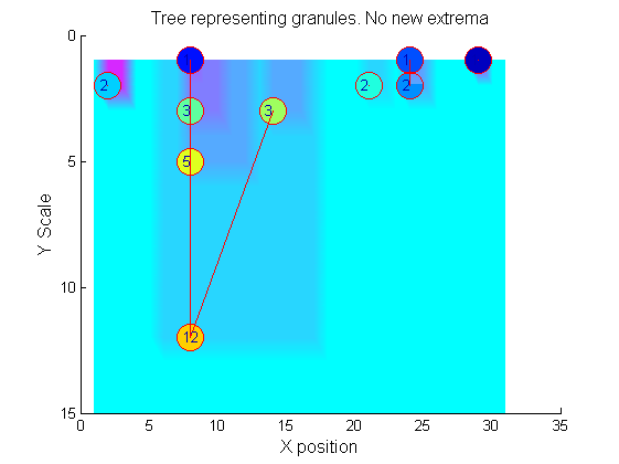
Label the granules
g=SIVND_m(X,maxscale,'o',1,'g',4);
g =   Number: 10
             area: [1 1 1 2 2 2 3 3 5 12]
            value: [6 1 1 2 5 1 1 1 1 1]
            level: [6 4 3 2 5 1 3 2 2 1]
        deltaArea: [5 2 1 7 3 12 2 2 7 19]
        last_area: [6 3 2 9 5 14 5 5 12 31]
             root: [29 8 24 24 2 21 8 14 8 8]
   PictureElement: {1x10 cell}
g.PictureElement
Columns 1 through 9
[29] [8] [24] [2x1 double] [2x1 double] [2x1 double] [3x1 double] [3x1 double] [5x1 double] [12x1 double]
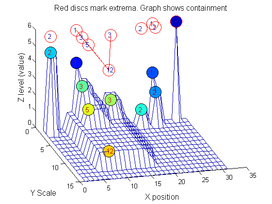
Tracing the granules through scale-space identifies candidate MSER's
We have candidate 1D MSER's
Which is the most stable?
This is a pragmatic judgement. Parameters might include
- how stable over scale (length)
- amplitude (value or level)
- a vector of amplitude over scale
- proximity to others
So far maxima. What about minima and more?
The filter (sieve) that finds maxima is a connect-set opening ('o' sieve). A 'c' sieve finds the connected-set closing, or minima. To work with minima we could:
- invert the signal, process it, and invert it back.
- OR, in this case, we could substitute a min for a max within SIVND_m.
YY=ones([length(X),1+maxscale]);
for scale=0:maxscale
    Y2=SIVND_m(X,scale,'c',1,'l',4);
    YY(:,scale+1)=Y2';
    Y1=Y2; % each stage of the filter (sieve) is idempotent
end
g=SIVND_m(X,maxscale,'c',1,'g',4);
This implementation also maintains lists of both maxima and minima throughout because there can be value in using the combined operators M, N, m
       switch type
           case {'o'} % opening, merge all maximal runs of less than scale with their nearest value
               data=ND_connected_set_merging(data,scale,type,verbose);
           case {'c'} % closing, merge all minima runs of less than scale with their nearest value
               data=ND_connected_set_merging(data,scale,type,verbose);
           case {'C'} % closing, invert-open-invert
               data.workArray=uint8(-double(data.workArray)+256);
               data.value=uint8(-double(data.value)+256);
               data=ND_connected_set_merging(data,scale,'o',verbose);
               data.workArray=uint8(-double(data.workArray)+256);
               data.value=uint8(-double(data.value)+256);
           case 'M' % Open close
               data=ND_connected_set_merging(data,scale,'o',verbose);
               data=ND_connected_set_merging(data,scale,'c',verbose);
           case 'N' % Close open
               data=ND_connected_set_merging(data,scale,'c',verbose);
               data=ND_connected_set_merging(data,scale,'o',verbose);
           case 'm' % recursive median
               data=ND_connected_set_rmedian(data,scale,'m',verbose);
           otherwise
               error('type not recognised it should be (m, o, c, C, M or N)');
       end


